Excel PowerPivot Tutorial

Importing Access Data into PowerPivot

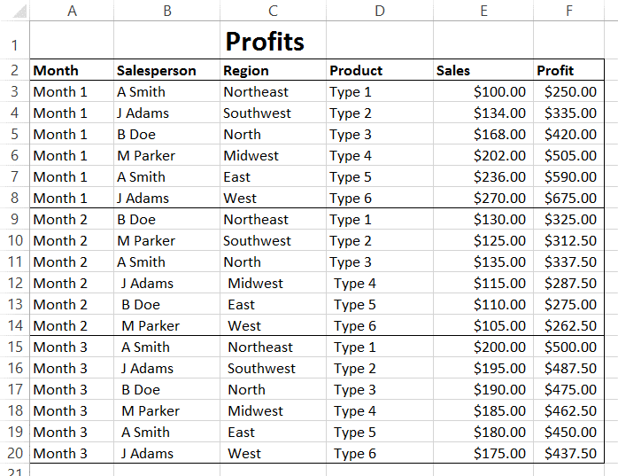
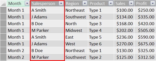
The sample Excel worksheet lists salespeople with accompanying data about the regions they work in, the products they sell, and their sales and profit amounts:

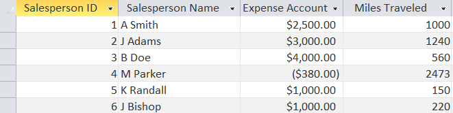
We have also created a simple database that includes information about the sales team and their expenses:

While both sets of information are useful, having them together would be even better.

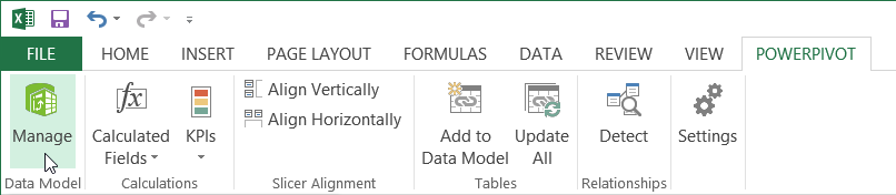
To start importing data from Access, click PowerPivot → Manage:

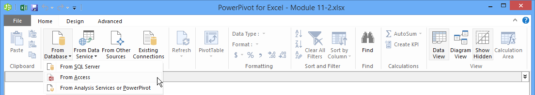
This action will open the PowerPivot window. Click Home → From Database → From Access:

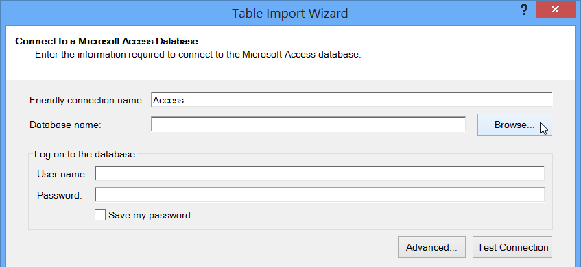
This action will open the Table Import Wizard. Click the Browse button:

The Open dialog will now be shown. Browse to the Exercise Files folder on your desktop.

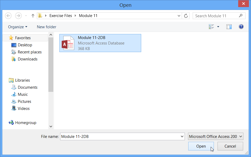
The database will now be listed inside the “Database name” text box:

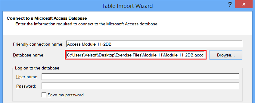
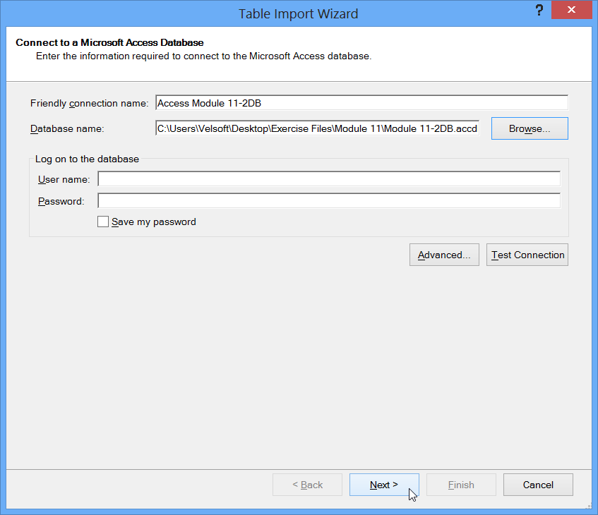
Logon credentials are not required for this database, so click Next:

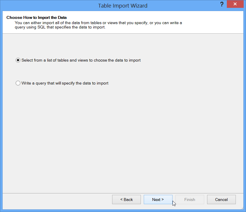
In the next stage of the wizard, you need to choose how to import the data. As this is a very simple database, ensure that the first radio button is selected. Click Next:

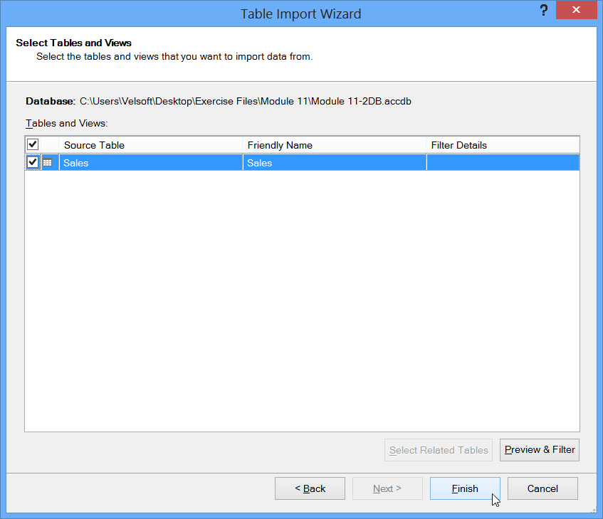
Next, you need to select what tables in the selected database that you would like to import. This particular database only has one table (Sales), so ensure that a checkmark is placed beside it and click Finish:

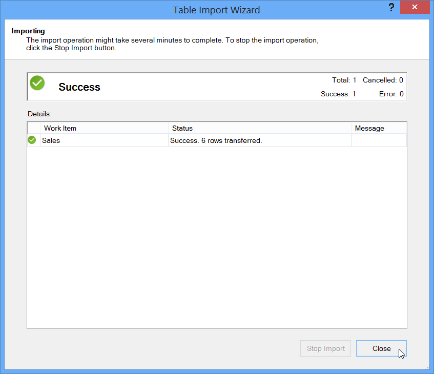
The data will now be imported. After the process is complete, click Close:

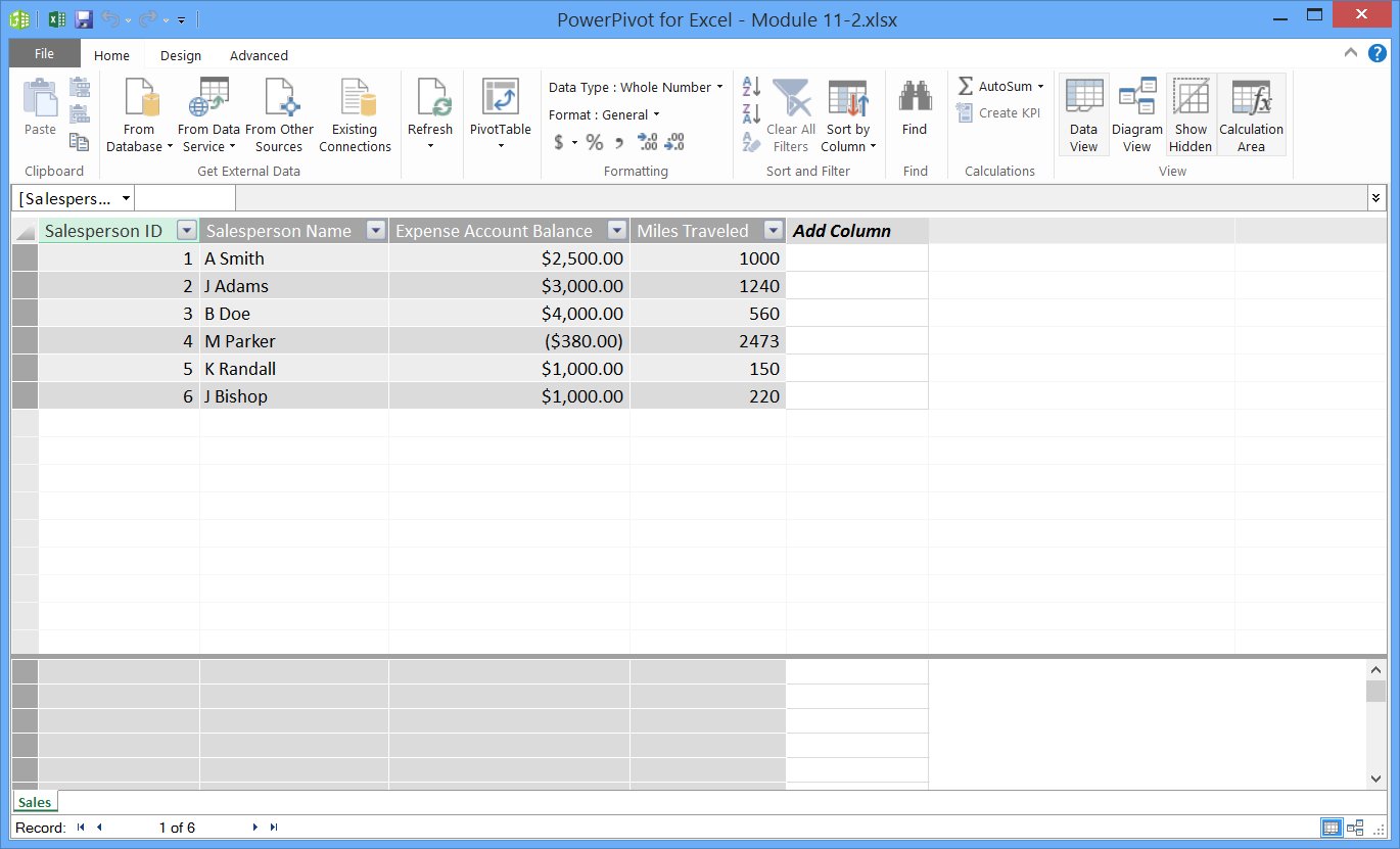
You will now be returned to the PowerPivot window where all of the imported data will be displayed:

Integrating Data with Relationships

In the sample workbook, data has been imported from two separate data sources. Now, we need to integrate this data. To do this, we need to create a relationship.

To start, open the PowerPivot window by clicking PowerPivot → Manage:

Ensure that the "Sheet1" tab is selected at the bottom of the PowerPivot window:

The data displayed here was imported from an Excel workbook. In particular, you can see that there is a column labeled Salesperson:

Switch to the Sales sheet by clicking on the Sales tab:

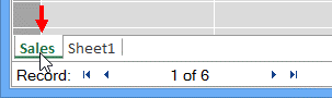
The data displayed here was imported from an Access database named Sales. Again, you will see a Salesperson column:

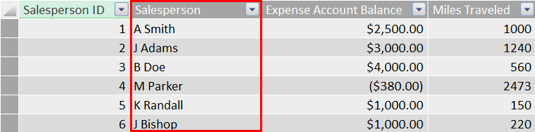
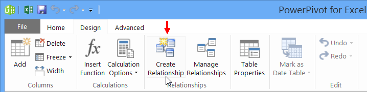
As the Salesperson field in each of these data sources uniquely identifies the same salespeople, it is ideal for integrating the data using relationships. To start, click Design → Create Relationship:

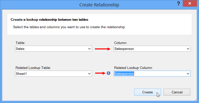
The Create Relationship dialog will be displayed:

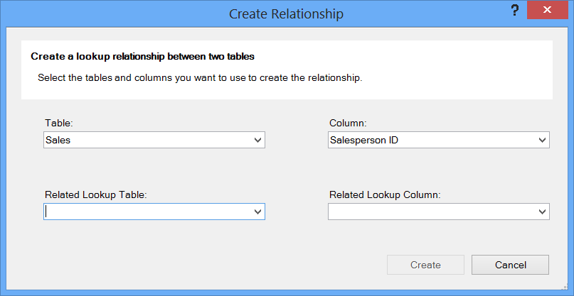
Using the controls in this dialog, you need to select the tables and columns you want to use to create a relationship. “Sales” should be listed in the top table field. Choose Sheet1 for the Related Lookup Table field. Ensure that both data sources use the same column (Salesperson). Click Create:

Now, in both data sources the Salesperson column header displays a relationship icon:

Creating a PivotTable with PowerPivot Data

Open the PowerPivot window by clicking PowerPivot → Manage:

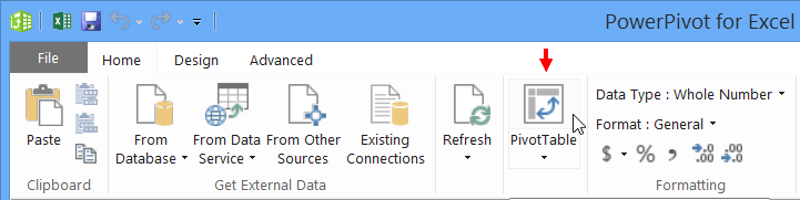
After a relationship has been created between PowerPivot data, you can create a PivotTable. With the PowerPivot window open, click Home → PivotTable (not the drop-down arrow):

This action will open the Insert Pivot dialog. For this example, ensure that the New Worksheet radio button is selected and click OK:

The new PivotTable will now be created in Excel. Inside the PivotTable Fields pane, you will see two sets of fields: Sales and Sheet1. Click on each item to expand them:

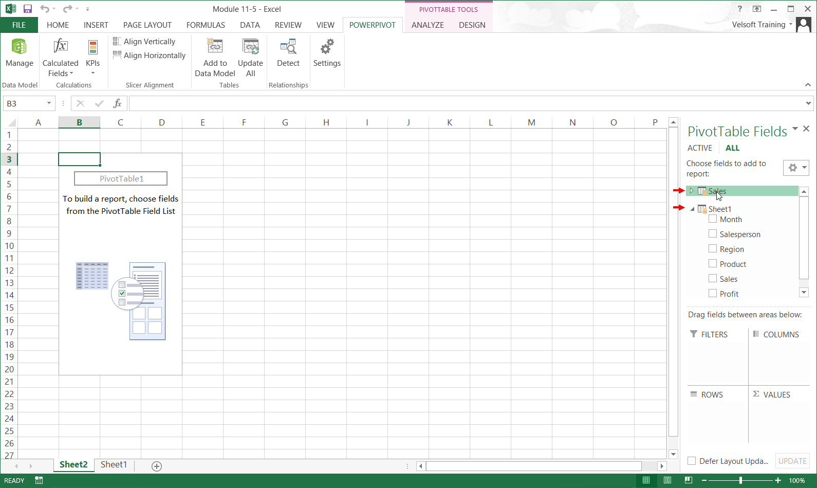
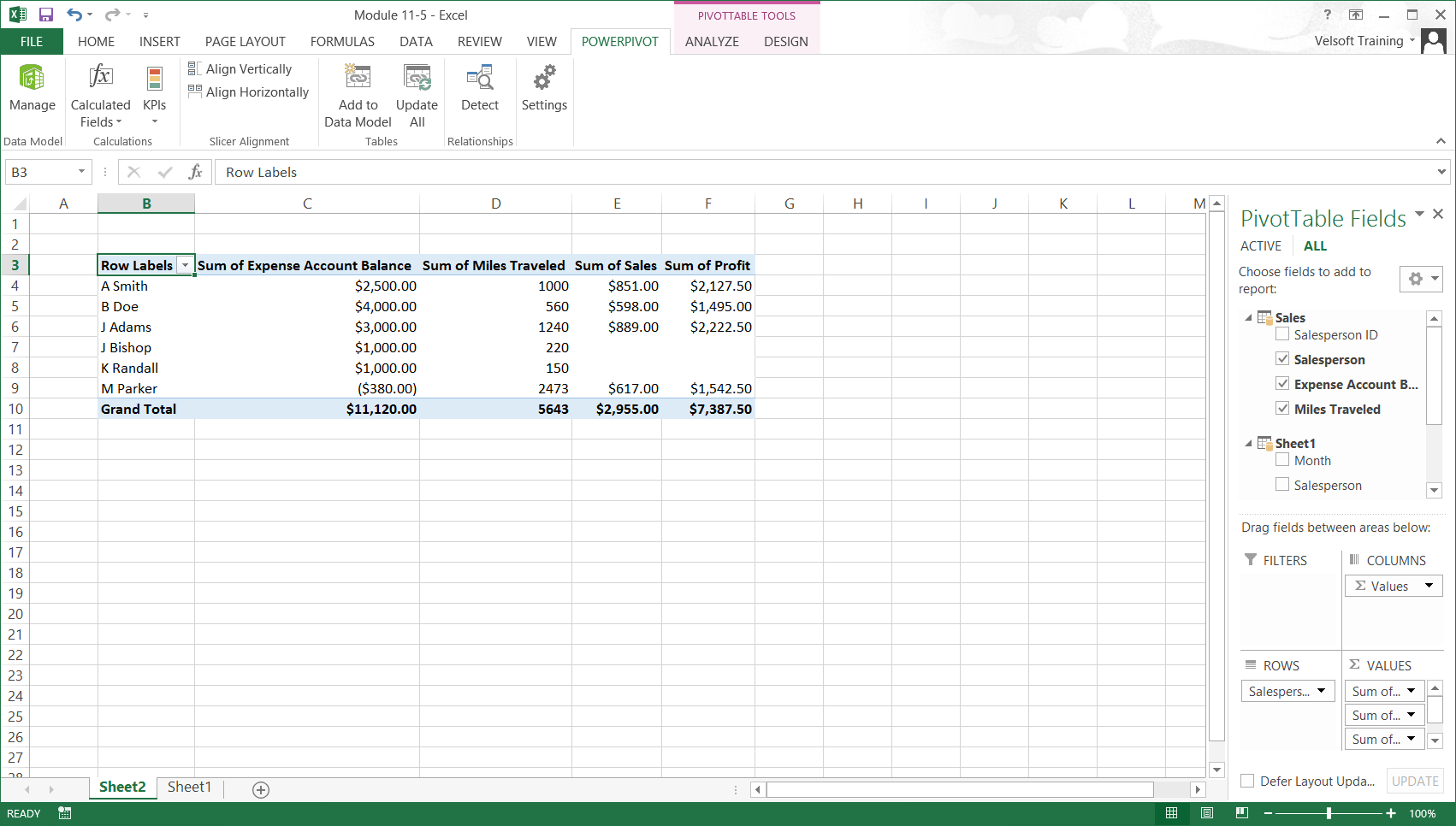
With both sets of fields now expanded, you can see all of the fields that are available. To add a field, simply click its checkbox. For this example, add Salesperson, Expense Account Balance, and Miles Traveled from the Sales field set. From the Sheet1 field set, add Sales and Profit. Now, you can see data from two different sources together in the same PivotTable:

You can work with this PivotTable as you would any other. If you need to access the data in this PivotTable, open the PowerPivot window by clicking PowerPivot → Manage:

If the data in the external source changes, you can refresh the data in the PowerPivot window by clicking Home → Refresh:

Then, you would need to refresh the PivotTable in Excel by clicking PivotTable Tools – Analyze → Refresh.

See all Seven Institute Excel training Options