Excel Introduction Tutorial
Working with Basic Formula
Formulas are mathematical expressions that operate on cell contents. When cells contain numerical data, you can perform multiple mathematical operations on the cell content as your worksheet requires. The results of these operations will be shown in the cell that contains the formula. Formulas can be simple, like adding two cell values, or quite complex, involving multiple mathematical operations.
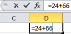
Formulae are always preceded by an equals sign ('='). Formulae can contain cell references (like 'A1'), numbers (like '23'), or even other functions (like 'SUM(B2:B9)'). Enter a formula by typing directly into a cell, or use the Formula Bar:
'=A1+23', '= d2-c2', and '=B10+b11/C6' are all valid formulae. Cell references are not case-sensitive.
If you include a cell reference in a formula (like '=B3*6'), and that cell reference itself contains a second formula (like '=B1+B2', stored in 'B3'), that second formula ('=B1+B2') will be evaluated first, and the result will be used in '=B3*6'.
If you include a cell reference in a formula (like '=B3*6'), and that cell reference itself contains a second formula (like '=B1+B2', stored in 'B3'), that second formula ('=B1+B2') will be evaluated first, and the result will be used in '=B3*6'.
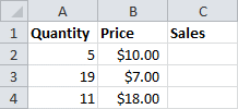
Consider the following worksheet. To calculate Sales, we must multiply Quantity by Price:
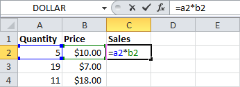
The formula '=A2*B2' will be entered into 'C2'. Note the colors that outline the cell references:
After the formula has been entered, press Enter to calculate the value:
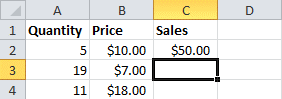
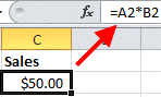
You can tell if a cell contains a formula by making it active. If there is a formula in the active cell, it will be shown in the formula bar:
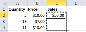
We know that Excel can use AutoFill in order to fill in a single value over and over or a sequential value. AutoFill also works with a formula. Select the cell that contains the formula you want to use, and click and drag the black square:
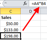
Excel will change the column/row references as necessary:
Formulas can contain multiple cell references from a single worksheet, or even references from different worksheets or workbooks. However, you can create a circular reference in Excel by referencing a cell that is dependent on the very cell that references it for a result.
For example, If 'A1' contains the formula '=10+B2', and 'B2' contains the formula '=A1-25', you have created a circular reference. Cell 'A1' cannot be resolved until Cell 'B2' is resolved, and vice-versa. You will be warned if Excel finds any such references.
Working with AutoSum
AutoSum
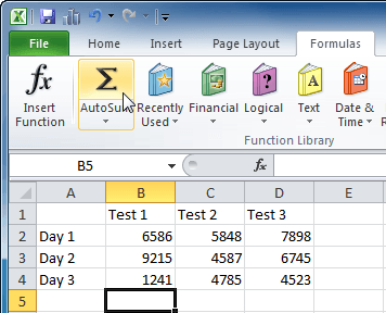
Most worksheets are used to calculate numerical or financial data, so Excel includes an AutoSum feature. This command will find the sum of a row or column of data,
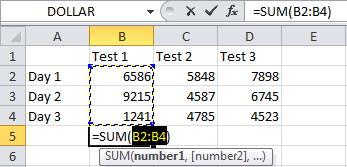
To use this command, click the cell immediately below (if summing a column of data) or to the immediate right (if summing a row of data) of the data you want to sum. Next, click Formulas → AutoSum:
Excel will scan the data in the column/row. The column or row of data to be summed will be highlighted by an animated border:
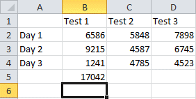
Press Enter to complete the AutoSum command:
AutoComplete
AutoComplete will help you enter data by automatically filling information in as you type, based on similar data in adjacent cells in the same column. This feature is enabled by default, and is very useful if you need to create a list of names or if you commonly enter the same types of data.
For example, if you typed “Alice” into a cell, pressed Enter, and then typed “a,” Excel would automatically fill in the remaining letters of “Alice”:

Just press Enter to accept the completion.
If you then typed the name “Arnold” into the same column, Excel will now be set up to AutoComplete either “Alice” or “Arnold.” However, you will need to type the second letter in order for Excel to determine which name you are entering:

AutoComplete has the potential to save you time when you type information, but sometimes it can get in the way. If you want to turn the AutoComplete feature off, click File → Excel Options → Advanced (tab on the left) → and uncheck “Enable AutoComplete for cell values:”
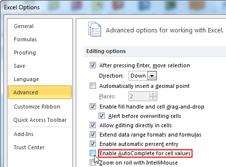
Click OK to accept the change. Excel will no longer use AutoComplete.
Working with Charts
We have certainly come a long way in our exploration of Excel! In the final two lessons of this section, we will explore the last major component to help you complete your workbook – how to create and modify charts. After completing these two lessons, you are well on your way to being able to create functional and attractive worksheets worthy of any quarterly report or boardroom meeting!
If you look at a large table of figures, it can be very hard to figure out what is happening with the data. Conditional formatting will help, but sometimes a picture really is worth a thousand words. Excel features powerful charting tools to help you create a more meaningful representation of your data. In this lesson, we will learn how to create, format, and manipulate a chart.
Creating a Chart
Office 2007 featured a number of interface improvements that were designed to help you get more things done quickly. Office 2010 continues with this new style of interface. The ribbon interface with bright, colourful icons was a step away from traditional menus and submenus. The interface changes weren’t necessarily loved by all, but they did make a lot of Office’s features more accessible to new users.
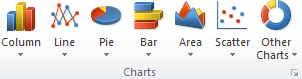
One of the major changes in Excel 2007 was the way that charts were created and handled. Excel 2010 uses these same changes. Instead of going through a chart wizard (a series of dialogs that let you choose options), a professional-looking chart can be created in just a few clicks. The main charting tools are found on the Insert tab:
Before you create a chart, consider the type of chart that you require. Pie charts and bar charts are good for showing comparisons. Line graphs can be useful for showing trends and plotting relationships between variables. Excel can produce three dimensional charts as well which may not be best for an internal report, but would be great for a Web site or promotional literature.
To create a chart, select the data that you want to use in the chart. This data should include some identifiers such as the row headings shown here. This is so Excel knows how to identify the data.
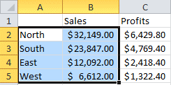
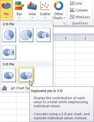
Now click Insert → Pie to view a list of possible pie charts. For this example, we will choose the exploded 3D pie chart:
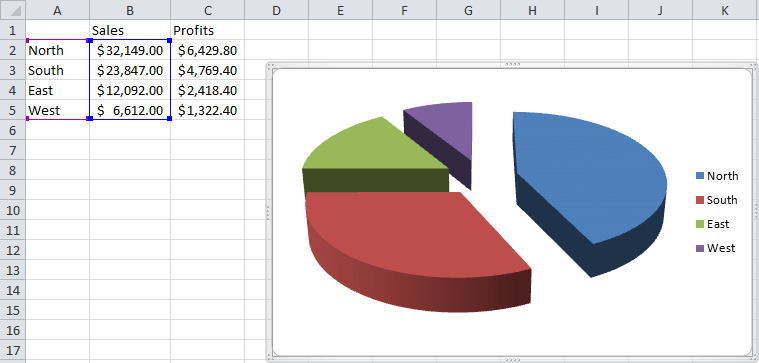
This action creates an exploded 3-D chart in the spreadsheet, showing comparative slices for the sales per region. Note that the data that was used to create the chart has been highlighted in the worksheet:
Styling Charts with the Design Tab
Once a chart has been created, it’s not set in stone – you can modify everything related to the chart, including size, colour, layout, visual effects, 3D effects, chart type, and even the data that was used to make the chart in the first place. In order to work with a chart, click the border surrounding the chart. Doing so will open a feature of Excel we haven’t explored in detail yet called contextual tabs:
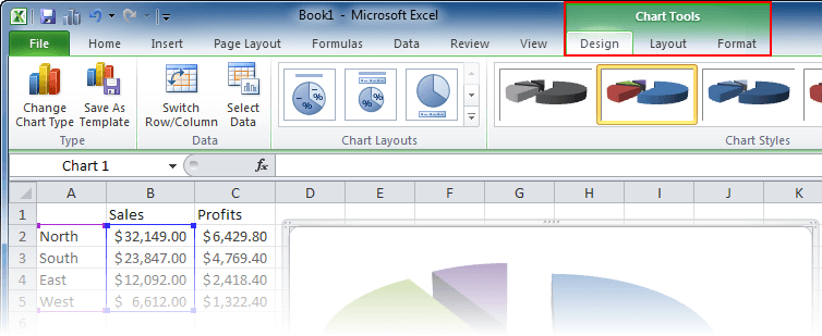
Contextual tabs appear when you are working with certain objects (i.e., you are working in context with them). There are three Chart Tools tabs: Design, Layout, and Format. These three tabs are only available when you are working with a chart. If you were to click elsewhere in the worksheet (deselect the chart), these tabs would disappear. Click anywhere in the chart again to bring them back.
See all Seven Institute Excel training Options