Excel Advanced Tutorial
Using a PivotTable in Excel
An important function of any spreadsheet program is to help you derive meaning from your data. An Excel PivotTable is a great tool for doing this. A PivotTable can help you get different perspectives as you analyze the relationships between the columns and rows of your data.
In this lesson you will learn what a PivotTable is and how to create one. You will also learn how to specify and rearrange PivotTable data.
What is a PivotTable?
A PivotTable is a powerful tool for exploring, summarizing, and analyzing information. A PivotTable helps you organize and manipulate the raw data in your spreadsheet to provide insight into patterns or relationships that might not be obvious at first glance. PivotTables also give you the power to summarize your data and view it in a different context, without changing the original content or structure of the data in the worksheet.
With a PivotTable, you can conveniently drag and drop columns of your data to different areas of the table to examine relationships or trends that may not be obvious in a traditional Excel table or database. (You can base a PivotTable on data in your current workbook or on external data.)
Rather than build several regular tables to explore how columns from an Excel worksheet relate to each other (or to see the data summarized in different ways), you can use one PivotTable to do the same thing. With a PivotTable, you can alter the table design without cutting, copying, pasting, or adjusting formulas and cell references. In short, PivotTables enable you to organize your data in meaningful ways, without doing a lot of tedious work. You could say that a PivotTable is like several data tables rolled into one.
Ideally, the source data for a PivotTable should be structured like a traditional Excel table or database. The source data should have a row of unique column headings distinguishing the data, and there should be no empty columns interspersed within the data. Also, blank rows in the source data can limit the usefulness of your PivotTable.
The following image shows a block of contiguous data that is ideal for a PivotTable:
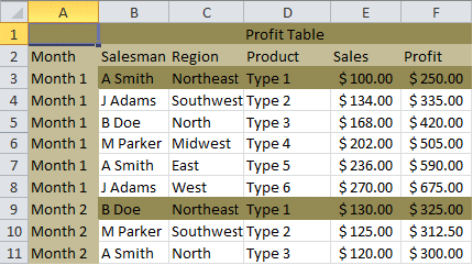
Notice that there are no empty rows or columns, and that every column of data has a unique label. When data like this is arranged as a PivotTable, you can quickly create views of the data that show (among other things)
- The profit for each product type across regions
- The sales figures for each product type across regions
- The profit for different product types by various sales people
These are only a few of the scenarios that you could generate with a PivotTable based on the given data.
Creating a PivotTable
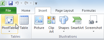
To create a PivotTable, select the range of data that you want to base the table on, and then click the PivotTable button on the Insert tab:
This will invoke the Create PivotTable dialog:
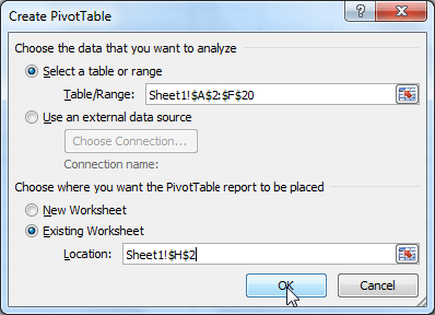
Notice that you are allowed to select data from an Excel table or range, or from an external data source. If you forgot to select the range before you opened the dialog, you can enter it now. If you choose the external data source option, you can base your PivotTable on data outside your current workbook (i.e. another workbook, or another source like an external database).
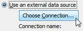
To start, select the “Use an external data source” radio button and click Choose Connection:
Then you will see a list of existing connections. A typical existing connection could be an MS query, or a connection you previously made to an Access data base for some other purpose. (There will be more on using external data later.)
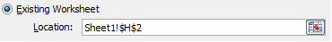
Once you select your data source, you can then choose to locate your PivotTable in an existing worksheet or a new worksheet. If you choose to locate it in an existing worksheet, you can specify the location for the upper left corner of the PivotTable by entering it directly into the Location field (as a cell reference), or by clicking the target cell with your mouse:
If you choose the New Worksheet option, your PivotTable will be located in the upper left corner of a new worksheet that will be added to your workbook.
Once you are ready, click OK to create your PivotTable:
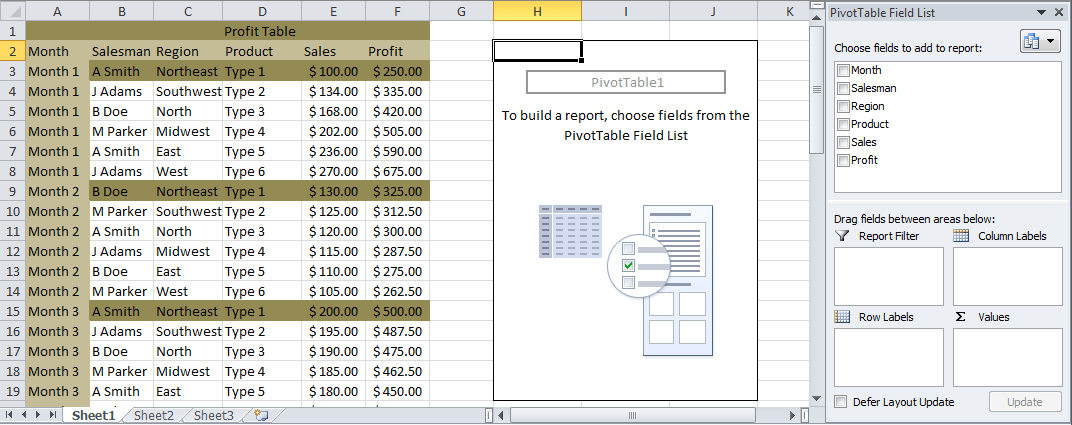
Above you can see a new PivotTable area and the corresponding PivotTable Field List placed in the existing worksheet that contains the source data.
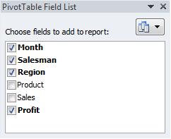
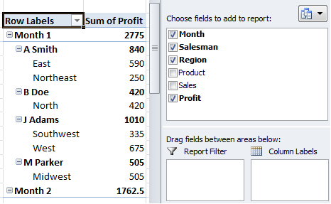
Once your PivotTable area appears, you can add information to it by placing checks in the boxes next to the fields in the PivotTable Field List. For this example, checks will be placed next to the Month, Salesman, Region, and Profit fields:
The PivotTable area will now be populated with the corresponding data:
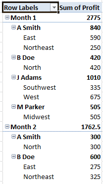
As you can see in the following image, the profit has been organized by Month. It has also been organized by Salesman, with a total profit for each Salesman in the Sum of Profit column. Because Region has been checked in the PivotTable Field List, you can also see a profit breakdown by region for each salesman:
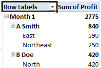
The following close-up view of the table tells us that the total profit for Month 1 is 2775. The Salesman A. Smith generated a total of 840 in profit with 590 from the East region, and 250 from the Northeast region:
As you can see, a PivotTable can provide more informative views of your data than a regular table.
Using LOOKUP functions in Excel
Excel provides two lookup functions that you can use to quickly retrieve information from data organized in a table. The functions are called HLOOKUP (horizontal lookup) and VLOOKUP (vertical lookup). In this lesson, you will learn how to use the VLOOKUP function to find data, limit VLOOKUP to an exact match, and find the closest match with VLOOKUP.
Understanding VLOOKUP and HLOOKUP
The VLOOKUP function will look in the leftmost column of a table for a value you specify. When it finds the value you specify, it will return a value that is located in the same row, a specified number of columns into the table. It is called VLOOKUP because it looks vertically down a column for a match, and then retrieves data from somewhere across that row.
HLOOKUP is similar, but it will look horizontally across the upper row of your table, and then retrieve data from somewhere below in the column. Since Excel is designed with more cells in the vertical direction than in the horizontal direction, and because vertical table design is more intuitive for most people, VLOOKUP is generally used more often than HLOOKUP.
Using VLOOKUP to Find Data
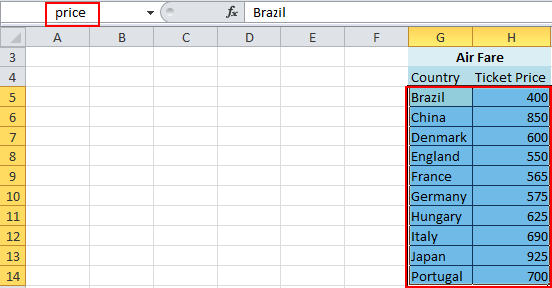
The best way to learn how lookup functions work is to look at an example. Here we have a table of ticket prices for flights to different countries. To simplify matters, the data range for the table has been given a defined name (“price”) that can be used in functions and formulas:
The arguments for the lookup function are: VLOOKUP(value to match, lookup table name or range, number of the column in the table containing the relevant data, true or false).
If we activate cell F1 and enter =VLOOKUP("England",price,2) into the formula bar, F1 will show the value 550:
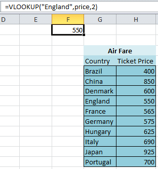
The lookup function looked vertically down the leftmost column of the lookup table (price) until it found a match for the text string “England.” The function then returned the value that is in the second (2) column of the table, in the row where the match was found. You should notice, that England, price, and 2 are the exact arguments used in the function.
For this example, the true or false argument was left out. The relevance of the true or false argument in the VLOOKUP function will be discussed shortly.

To use the VLOOKUP function correctly, you need to have your spreadsheet data laid out properly in table form with at least two columns. The first column in the table will contain the keys (identifiers that the VLOOKUP function will examine for a match). In the example just shown, the keys are the names of the countries. This first column can be referred to as the lookup column.
The other columns in your table will contain data that corresponds to the column of keys. Your table can be several columns wide, and you can specify which column VLOOKUP will retrieve data from by putting a number corresponding to the given column in the function. In the previous example, we wanted VLOOKUP to return the ticket price, so we used the number “2” (for the second column) as an argument in the function. If your table has 10 columns and you want to return data from the ninth column, you would use 9 as an argument.
You do not have to use text values (like the country names used here) in your lookup column. If it is more appropriate, numbers or dates will serve just as well.
If you want some help when you are using VLOOKUP, use the Insert Function dialog:
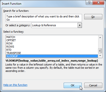
You will find the VLOOKUP function in the Lookup & Reference category. If you click OK in the Insert Function dialog, you will see the helpful Function Arguments box:
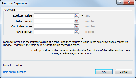
Simply enter the function arguments in the fields provided.
Working with Names and Ranges in Excel
Working with data isn’t always easy. A complex formula involving several cell ranges can be difficult to understand, and individual cells that contain important data can be hard to find on a large worksheet. Cell references like D5:D22 or A33:C660 don’t communicate anything about the data they contain.
To overcome this issue, Excel enables you to create meaningful names for cells and ranges. In this lesson, we will learn what cell and range names are and how to use them. We will also cover nonadjacent ranges and learn how to take advantage of Excel’s very handy AutoCalculate feature
What are Range Names?
Range names are meaningful labels that you can assign to individual cells or cell ranges. You can use a range name anywhere you would use a cell reference or cell range reference. This means you can use a name like “Employees” to describe a range of cells rather than their reference (like C2:C55).
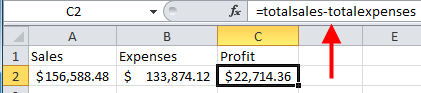
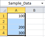
For example, consider the following worksheet. Cells A2 and B2 have been given names and those names have been used in a formula in cell C2:
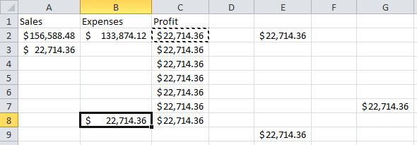
As an added bonus, range names use absolute cell references. This means that if you copy a formula or use AutoFill while using named ranges, the formula will maintain its original cell references:
Range names make formulas much more readable, improve worksheet clarity, and greatly improve worksheet organization. Range names can even help in overall design of your worksheet.
Most small worksheets are usually constructed by filling a sheet with data and then performing calculations. However, range names enable you to complete a sheet by doing the opposite: constructing formulas and then adding the data. When you are designing your worksheet, you can create formulas using names instead of traditional cell references, and then define the names for the corresponding ranges as data becomes available.
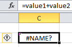
For example, here is an empty worksheet with a defined formula but no defined names, which results in a #NAME error. This error will remain visible until both “value1” and “value2” have been defined:
Defining and Using Range Names
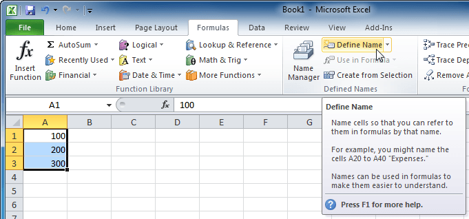
Now that you understand the purpose of ranges, let’s explore how to use them. To define a range name, select either a single cell or cell range and click Formulas → Define Name:
This will display the New Name dialog box. Give the cell or range a name, select which part(s) of your file will be able to use this name, and add a comment if you wish. By default, the active cell/selected cells will already be filled in at the bottom, but you can click the Change Cells button to define a new range:
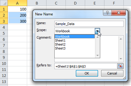
- Names cannot begin with a number. You can use only letters or underscores.
- Names cannot have spaces.
- Names cannot be the same as built-in names included with Excel.
- All names must be unique to the workbook.
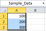
Click OK to apply the name. Once a name has been applied, you can see the name in the name box (next to the formula bar), provided you have selected the correct cell/range that has the name:
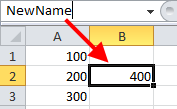
You are free to modify the data in the range however you like. Even if you add extra rows or columns to the worksheet, the name will still apply:
You can also name a cell or range by selecting it and then typing a name in the name box:
Click the pull-down arrow to the right of the name box to display a list of range names used in the current worksheet:
Using these range names will make your formulas and functions much clearer, especially if your work is to be passed on to others. It is much easier to remember and type the name of the range rather than specific cell references.
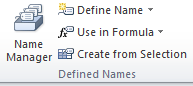
Defined Names Commands
Let’s take a moment to explore the commands within the Defined Names group of the Formulas tab:
Name Manager
Click this command to open the Name Manager dialog box:
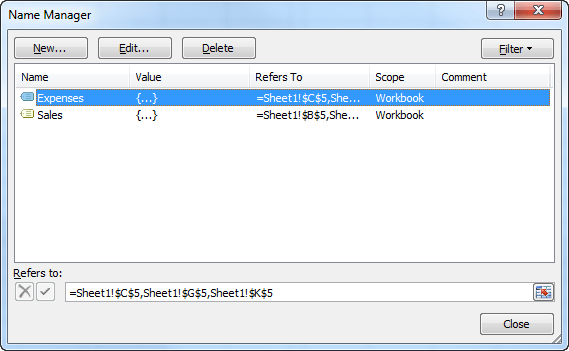
The Name Manager offers you a single location to view and manage all of the range names in your workbook. Use the three buttons at the top to create a New range or Edit/Delete the currently selected range.
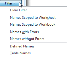
Use the Filter command to show only the ranges based on the current criteria:
When you have finished using the Name Manager, click Close.
Define Name
Select a cell or cell range and click this command to define a new name. Give the range a name, decide which worksheet will use this name (by default, the whole workbook can use a range name), add a comment, and manually edit the cell range if necessary.
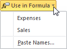
Use in Formula
Click this command to insert any defined range name in the current cell:
Create from Selection
Excel can automatically create a range name using this command. Many people label their data in the top left-hand corner, so this command can examine a selected range of cells and determine a name from Words that are selected in the range.
Consider the following range:
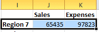
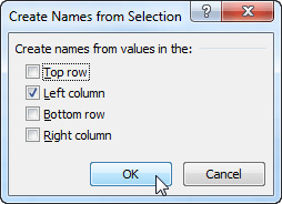
Click Create from Selection to show the Create Names from Selection dialog box. In this example, there is text in the leftmost cell, so Excel suggests that this range should be named based on the left column. Click OK to name this range “Region 7:”
See all Seven Institute Excel training Options