Excel PivotTable Tutorial
Creating a Basic PivotTable
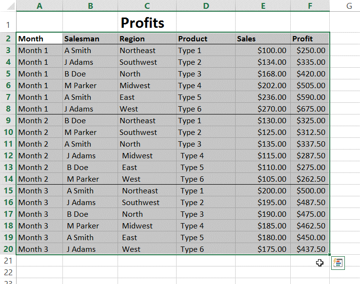
PivotTables are designed to make it easy to tabulate and summarize data in your worksheet. In order to create a PivotTable, you first need to select the range of data that you want to base the table on. For this example, select the cell range A2:F20:
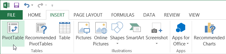
Next, click Insert → PivotTable:
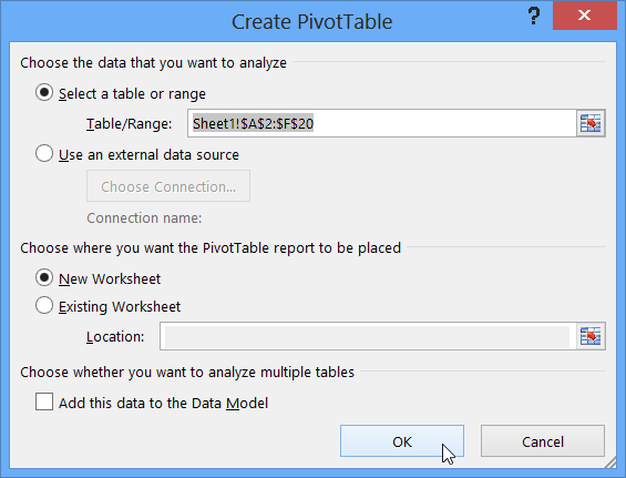
This action will open the Create PivotTable dialog box:
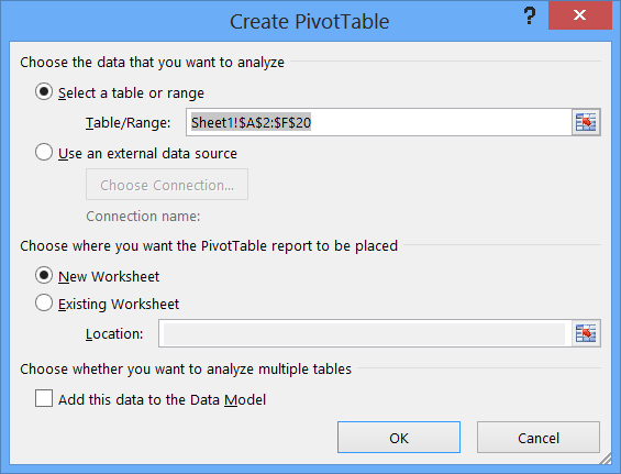
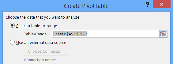
The range of data that you just selected will be displayed within the Table/Range text box:
You also have the option of selecting data from an external data source (such as another workbook or even a database) by selecting the "Use an external data source" radio button and clicking Choose Connection.
Lower in the Create PivotTable dialog, you can see options to choose where the new PivotTable will be placed:
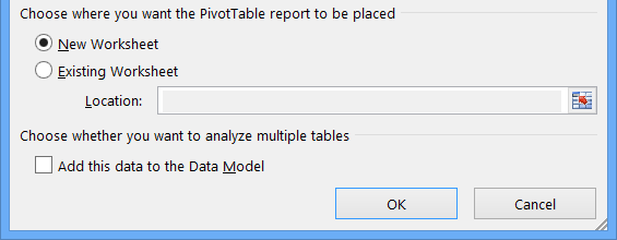
For this example, leave the default settings unchanged and click OK:
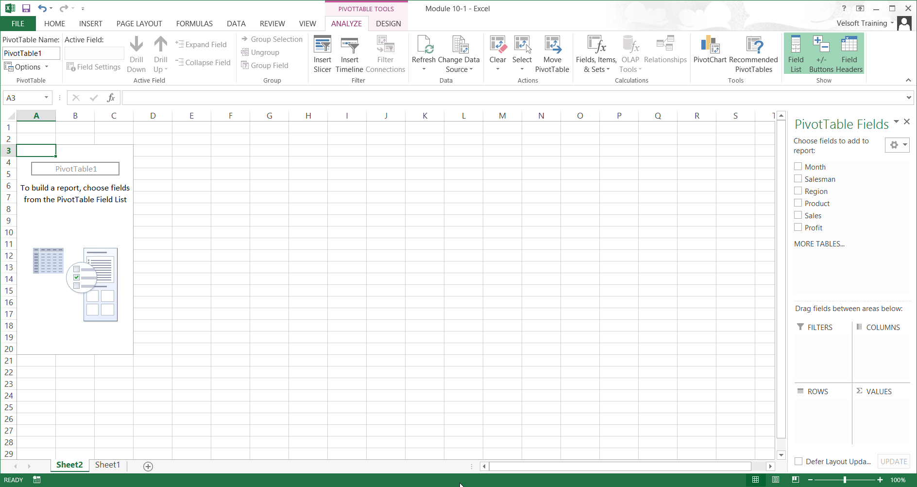
A new PivotTable will be created on a new worksheet. This worksheet will automatically be displayed with the PivotTable area in the upper left-hand corner:
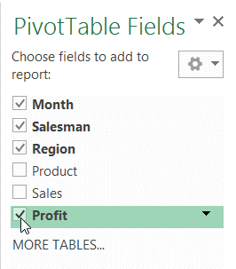
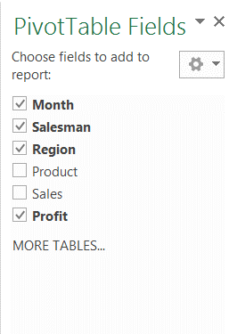
Now that the PivotTable has been created, you can start adding information to it. Do this by checking the boxes beside the Month, Salesman, Region, and Profit fields in the PivotTable Fields pane:
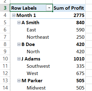
The PivotTable will now be populated with the data that you selected:
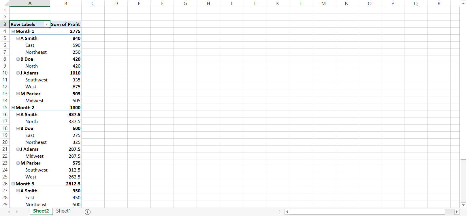
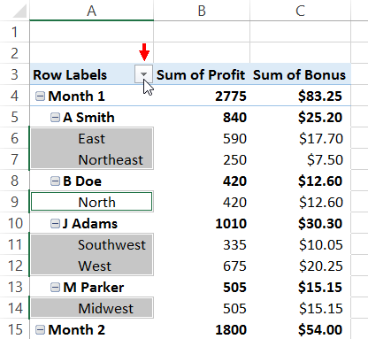
As you can see in the following image, the profit has been organized by Month and by Salesman, with a total profit for each Salesman in the Sum of Profit column. Because Region has been checked in the PivotTable Fields pane, you can also see a profit breakdown by region for each salesman:
Using the PivotTable Fields Pane
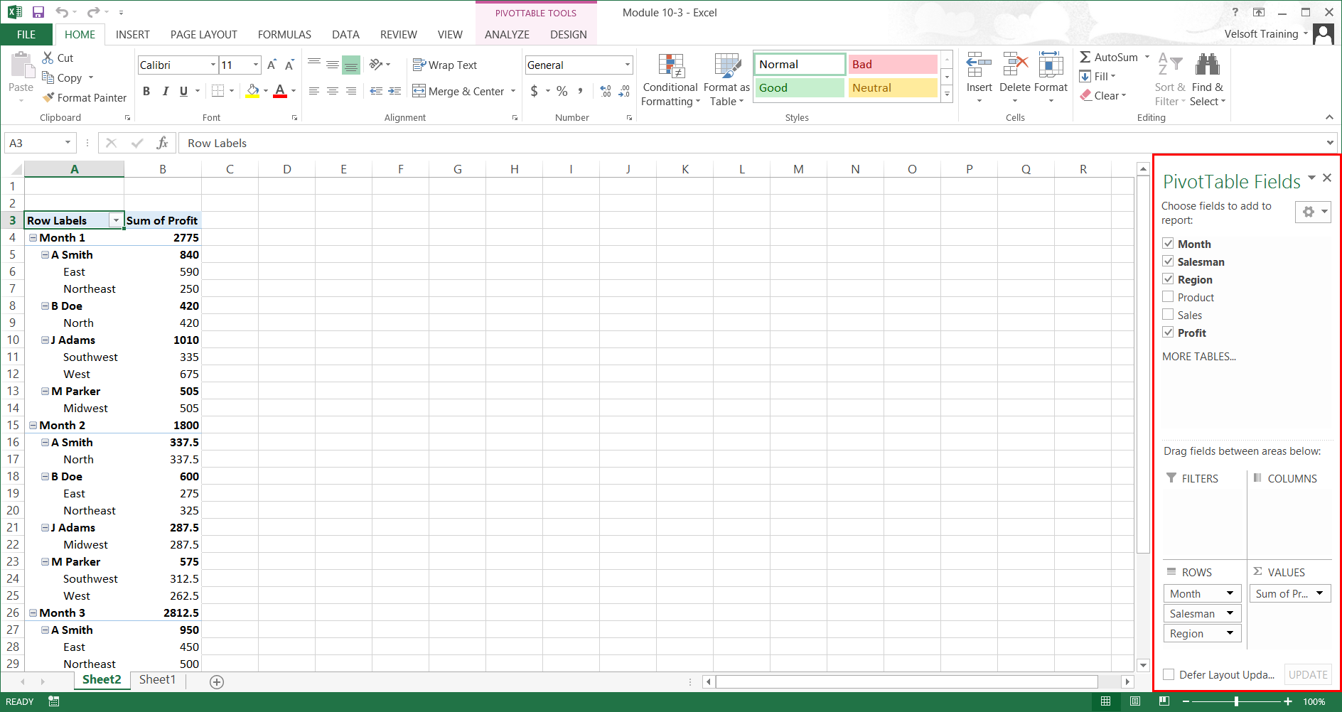
The PivotTable Fields pane will be displayed once a PivotTable has been inserted. In the sample workbook, you can see it on the right-hand side of the Excel 2013 window:
If you cannot see this pane, click PivotTable Tools – Analyze → Field List:

The PivotTable Fields pane is divided into two primary sections:
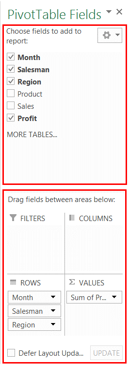
The Fields section lists all of the various fields that you can add to the PivotTable. If a field has a checkmark beside it, this indicates that the field is already part of the PivotTable. In this example, you can see that Month, Salesman, Region, and Profit are all part of the PivotTable:
In the upper right-hand corner of this section, you can see the Tools drop-down command. Click this command to see different layout options for the PivotTable Fields pane:
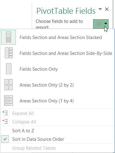
As you can see, there are five preset layouts that you can choose from. To apply a new layout, click on one of the options listed. (Generally, it is best to choose a layout that contains both the Fields and Areas sections.) Click the Tools button again to close the menu.
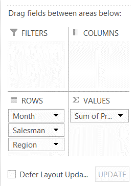
The Areas section of this pane allows you to specify what fields appear as filters, columns, rows, and values:
Sorting Pivoted Data
To sort data in a PivotTable, click the arrow in the top left-hand corner of the table:
This menu will feature a few sorting options:
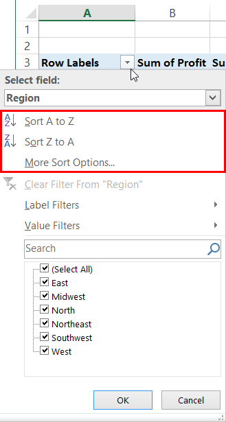
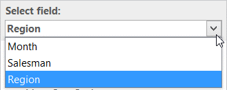
Choosing the "Sort A to Z" option will sort the table rows in ascending order. Choosing "Sort Z to A" will sort the table rows in descending order. If there are multiple row fields in the table, you can specify which field to sort using the “Select Field” drop-down menu:
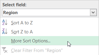
For expanded sort options, click More Sort Options:
This action will open the Sort dialog:
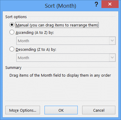
Again, you will see options to sort data in ascending or descending order. In addition, once you select a radio button, you can click the corresponding menu to choose a field to sort by. There is also a button on the bottom of the Sort dialog labeled More Options. If you click this button, another dialog will appear with an AutoSort option. If this option is selected, the data will be sorted automatically every time the PivotTable is updated.
See all Seven Institute Excel training Options