Excel Intermediate Tutorial

Working with Tables in Excel

As we have seen in the last two sections, Excel is capable of doing just about anything involving data calculation. In this lesson, we will introduce another interesting feature: Excel is a very capable program for managing small databases.

In this lesson, we will introduce tables, a great feature for separating data in a worksheet and the starting point for all databases, large and small.

What is a Table?

A table is a specially designated range of information that has added functionality that other cell ranges do not have. You can have multiple tables per worksheet, and tables can be as large or small as the amount of data you want to work with. We have already seen some worksheets that use tables, such as the personal budget template. In fact, this worksheet is composed almost entirely of tables:

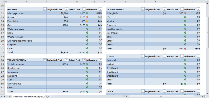
A table is made from adjacent columns of data, with a unique label or heading for each column. Each row in the table should have entries organized according to the column headings. Remember, each worksheet has a lot more rows than columns. This design is well suited for data organized in long, adjacent, list-like columns. You can make a table with empty rows or columns if required, but this is not recommended.

Creating Tables

Tables are made in one of two ways: by selecting and converting existing data, or by creating a blank table and filling in the information as required. In addition, tables can only be created from adjacent data.

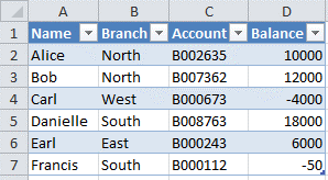
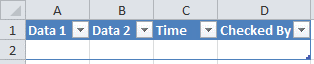
Let’s start by looking at how to mark existing data as a table. Consider the following well-defined data:

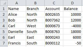
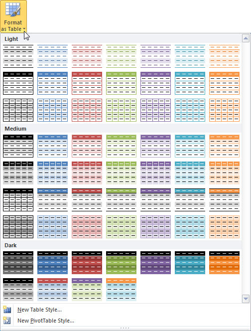
To create a table using existing data, select all data and column headings and then click Home → Format as Table → choose a table style:

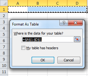
The Format As Table dialog box will appear and include the selected range of cells. Note the absolute cell references:

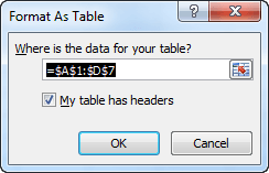
By default, “My table has headers” is checked whenever you select more than two rows of data. Make sure the cell range shown is correct and then click the OK button to create the table:

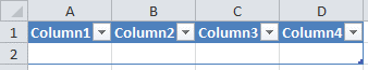
To create a table from scratch, click and drag the number of cells you will need in your table and then click Format As Table:

Click OK to apply the table. The first row will contain column headings and the second row is ready to accept new data:

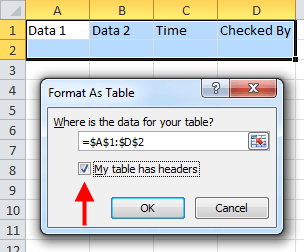
If you know what your column names need to be but don’t yet have any data, select the column names and the next row down before clicking Format As Table:

Using the IF Function

Logic operations play a big part in Excel’s functionality. One function in particular, the IF function, is very useful. You can use this function to calculate different values depending on the evaluation of a condition. The structure of an IF function is as follows:

IF(logical_test, value_if_true, value_if_false)

IF functions are called conditional functions because the return value will depend on whether or not a specific condition was satisfied. Consider the following function:

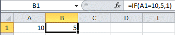
IF (A1=10, 5, 1)

If the value in A1 equals 10, then 5 is returned. Otherwise, 1 is returned. Let’s look at how this works in Excel once we start to fill in the equation:

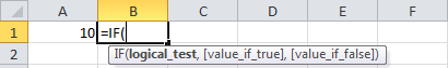
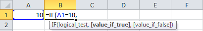
The small box beneath the function will tell you what you need to enter. Right now, the next expected argument is a logical expression. In this case, we want to test if A1=10, so we will add that and then a comma:

Now we will add the two remaining values and a closed parenthesis:

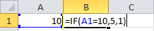
The formula is now complete, so press Enter to complete the calculation:

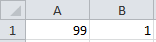
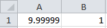
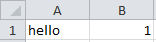
Anything other than 10 in A1 will calculate as false and make Excel return 1:

Working with Nested Functions

Excel allows you to use functions within functions. This is called “nesting.” Excel lets you have up to 64 nested functions in a single calculation. Consider the following worksheet:

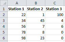
Data has been recorded in three different locations. If you wanted to find the average of all values, you could use the AVERAGE function to calculate the average at each station and then find the average of those three values. However, there is a way to compute this value in one step by using nested functions:

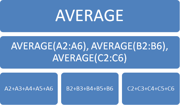
AVERAGE(AVERAGE(A2:A6), AVERAGE(B2:B6), AVERAGE(C2:C6))

Whenever Excel encounters nested functions such as this, it examines the whole statement and then looks at the order of operations to determine what need to be done first. Nested functions behave like a hierarchy. In this case, the outside AVERAGE function depends on the inputs of the three inside average functions. The three inside averages are then passed to the outside AVERAGE function and the final result is then calculated.

Here’s another way to look at the way the same nested function is calculated. This formula is calculated from the bottom to the top:

It can be tricky to wrap your head around the thinking behind nested functions. Just remember to take it one step at a time, figure out what needs to be calculated in what order, and be careful with your parentheses!

Breaking up Complex Formulas

As you can see, Excel is capable of doing a lot in a single cell. But what you might not be able to see is how the formula actually works! Therefore, Excel takes a cue from computer programmers and allows you to add line breaks to a formula.

Consider the following worksheet that contains test scores. The students were given a quiz that was marked out of 10:

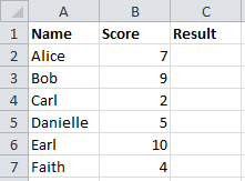
The teacher wants to add a description to each student’s score based upon their mark. If the student scores 8 or higher, their mark is Very High, if they score 6 or higher their mark is High, etc. The teacher ends up creating the following nested formula which will be AutoFilled for every student’s mark:

IF(B2>=8, “Very High”, IF(B2>=6, “High”, IF(B2>=4, “Average”, IF(B2>=2, “Low”, “Very Low”))))

This statement is correct but it’s not very easy to read. If we add a few line breaks, the statement should be much easier to read:

IF(B2>=8, “Very High”, 
    IF(B2>=6, “High”, 
        IF(B2>=4, “Average”, 
            IF(B2>=2, “Low”, “Very Low”))))

If the mark is 8 or higher, the rank is Very High. If it’s not, Excel will continue attempting to calculate the mark until the statement is found to be true or false.

To add these line breaks, click and drag the divider between the formula bar and the cells down a bit and then press Alt + Enter to add a line break at various points within the formula:

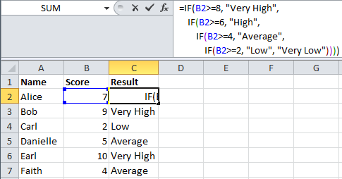
Look carefully at the formula bar: Excel automatically colors the parenthesis to make sure you have the correct number of opens and closes.

See all Seven Institute Excel training Options